The Ross orogen: An ancient continental arc exposed in the Transantarctic Mountains
Graham Hagen-Peter
University of California, Santa Barbara
An introduction to the Transantarctic Mountains and the Ross orogen
The Transantarctic Mountains form the boundary between the Archean and Proterozoic East Antarctic Craton and younger accreted terranes of West Antarctica (Fig. 1). This mountain belt formed through Cenozoic extension, but older metamorphic and igneous rocks associated with the convergent Ross orogeny are exposed in the up-thrown rift shoulder. Deformation, metamorphism, and magmatism in the Ross orogen are associated with convergence and subduction of paleo-Pacific oceanic lithosphere beneath East Antarctica during the late Neoproterozoic–early Paleozoic. The middle- and upper-crustal levels of the eroded Ross magmatic arc are exposed over thousands of kilometers along the Transantarctic mountains and provide an excellent opportunity to study the intrusive components of a subduction related magma system. We are studying the orogenic history, from pre-magmatic deformation and metamorphism through post-orogenic magmatism, of the southern Victoria Land region (Fig. 1).
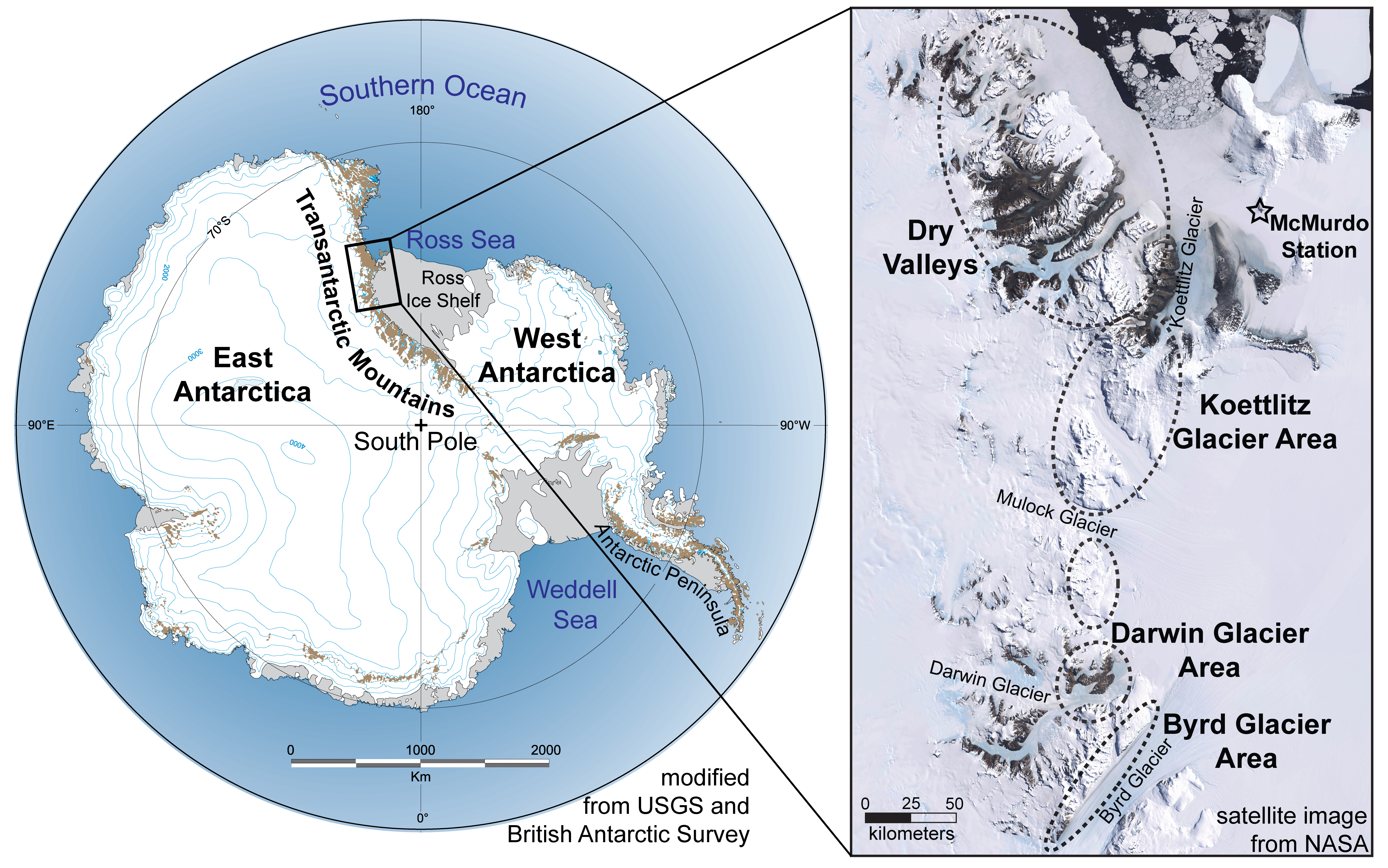
Figure 1. The Transantarctic Mountains span thousands of kilometers across the Antarctic continent. Metamorphic and igneous basement is well exposed (by Antarctic standards) in the southern Victoria Land region (area of the satellite image). The ellipses outline the different areas that we have focused on.
The challenges (and advantages) of fieldwork in Antarctica
As one can imagine, doing geologic fieldwork in Antarctica has its difficulties. First of all, the continent is very remote. So how do we get there? Our study areas are just inland from the McMurdo Station on Ross Island (Fig. 1), and so this station was a practical home base for us during our two field seasons on “the ice”. We flew from Christchurch, New Zealand to McMurdo on a U.S. Air Force C17 jet. This journey is surprisingly quick (~ 5 hours) on one of these aircraft. After an incredibly smooth landing (perhaps owing to the packed snow and ice runway), a group of seasoned technical- and support-staff and bewildered scientists step out onto the ice, many for their first time (Fig. 2).
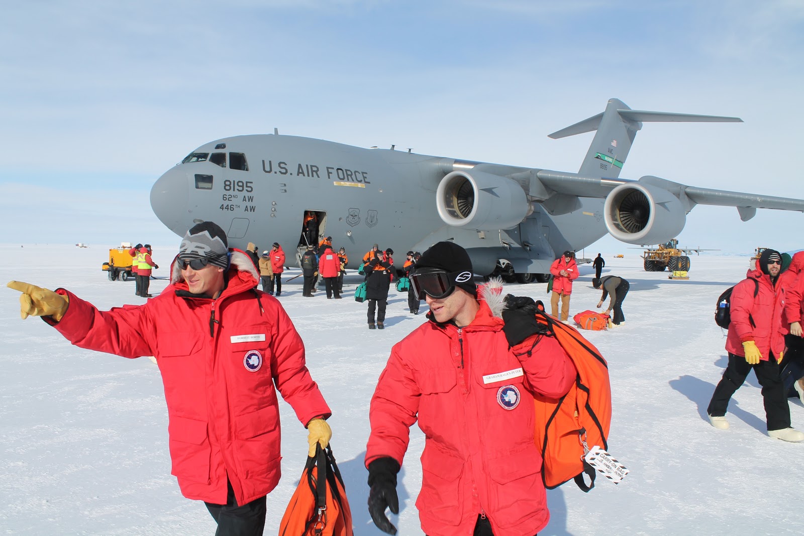
Figure 2. Exiting the C17 after landing on the ice runway.
At the beginning of each field season, we spent about one week at McMurdo prepping for the fieldwork. We gathered the necessary supplies for two months in a field camp and participated in various technical trainings. Perhaps the most memorable of these trainings was “Happy Camper”, required of all personnel who leave the station for fieldwork. Under the beautiful and looming Mt. Eribus, the southernmost active volcano in the world, we learned how to build snow walls around a camp, erect scott tents, light a stove in windy conditions, and what not to do in a staged search-and-rescue scenario in white-out conditions (Figs. 3;4).
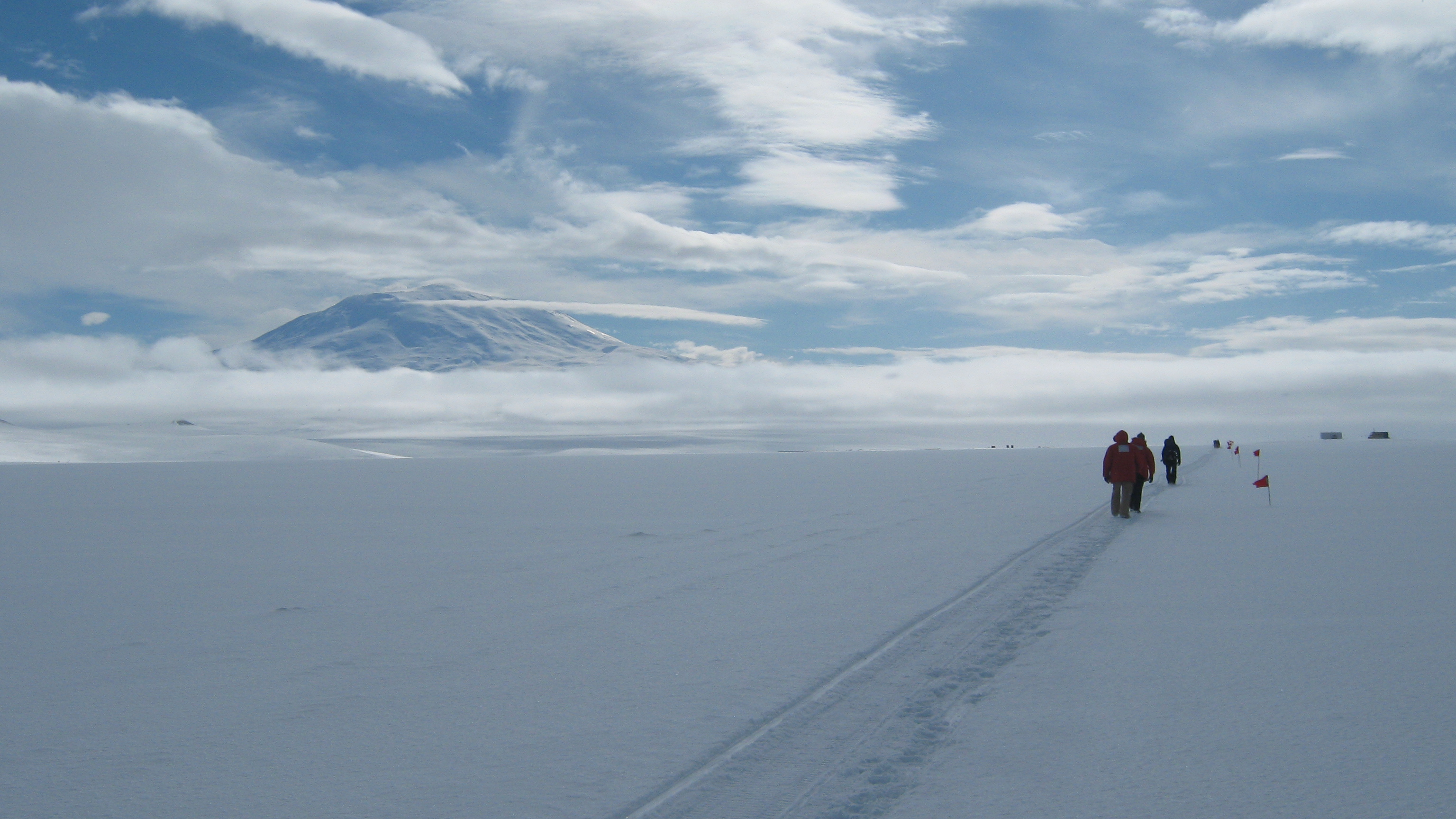
Figure 3. Happy Camper participants follow the flag-marked route to the training hut. Mt. Eribus looms in the background.

Figure 4. Several participants at the “Happy Camper” campsite dig snow trenches, while others set up tents. Red and green flags mark safe routes in case of poor-visibility conditions.
Once all of our gear and food was in order, we were transported to our field area, either by helicopter or a small airplane. Our team consisted of three or four geologists and sometimes a field guide. We would set up a small field camp to work out of for several weeks. The camps typically consisted of one large “endurance” tent for cooking and two smaller “scott” tents for sleeping (Fig. 5). We would construct a bathroom by digging a pit and surrounding it with snow walls. The snow walls were important for blocking wind, but the pit would fill up with snowdrifts, requiring regular shoveling (Fig. 6). We used a small solar panel to recharge the batteries in our satellite phones, HF and VHF radios, and ipods, but the camps were otherwise without power or heat.
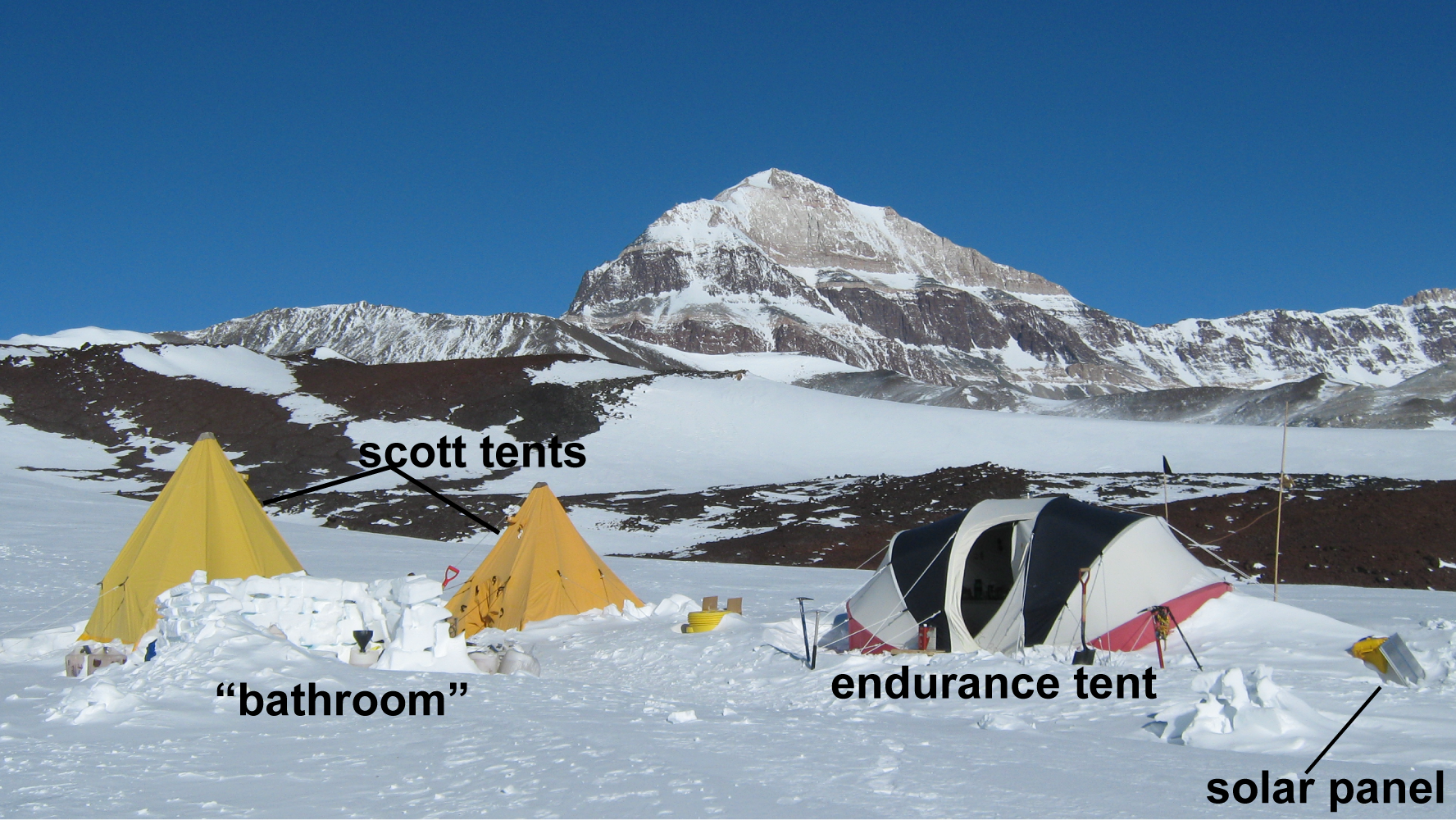
Figure 5. A typical field camp consists of several scott tents and an endurance tent. Full pee jugs surround our “bathroom” (yes, we take out all waste). We learned the hard way that an overfilled jug would spill as it froze and expanded.
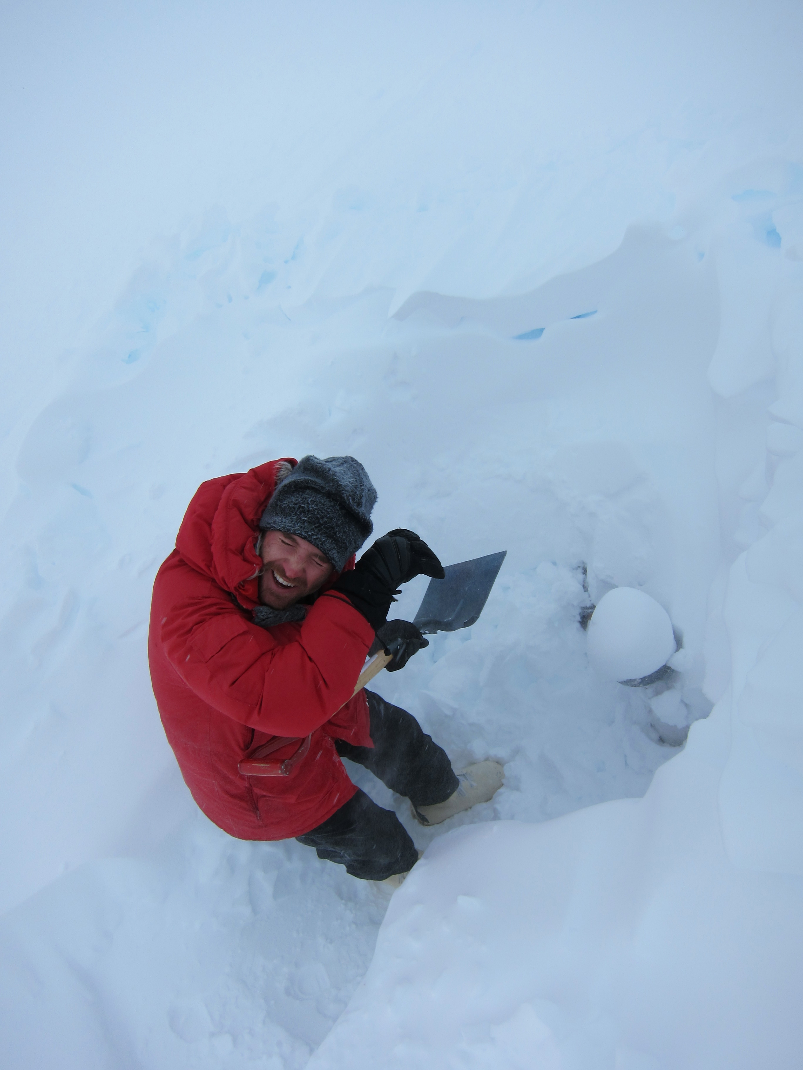
Figure 6. Shoveling out a drift-filled bathroom.
We would typically move these camps once or twice in one field season, but spending so much time in a small camp with two or three other people can cause cabin fever. I found that one of the best ways to stay sane was to cook elaborate meals often! We ate surprisingly well in the field, with fare including cornish hen in Thai peanut sauce and home-made cinnamon rolls! We also ate a lot of candy to keep up with our increased caloric needs! (Figs. 7;8;9)
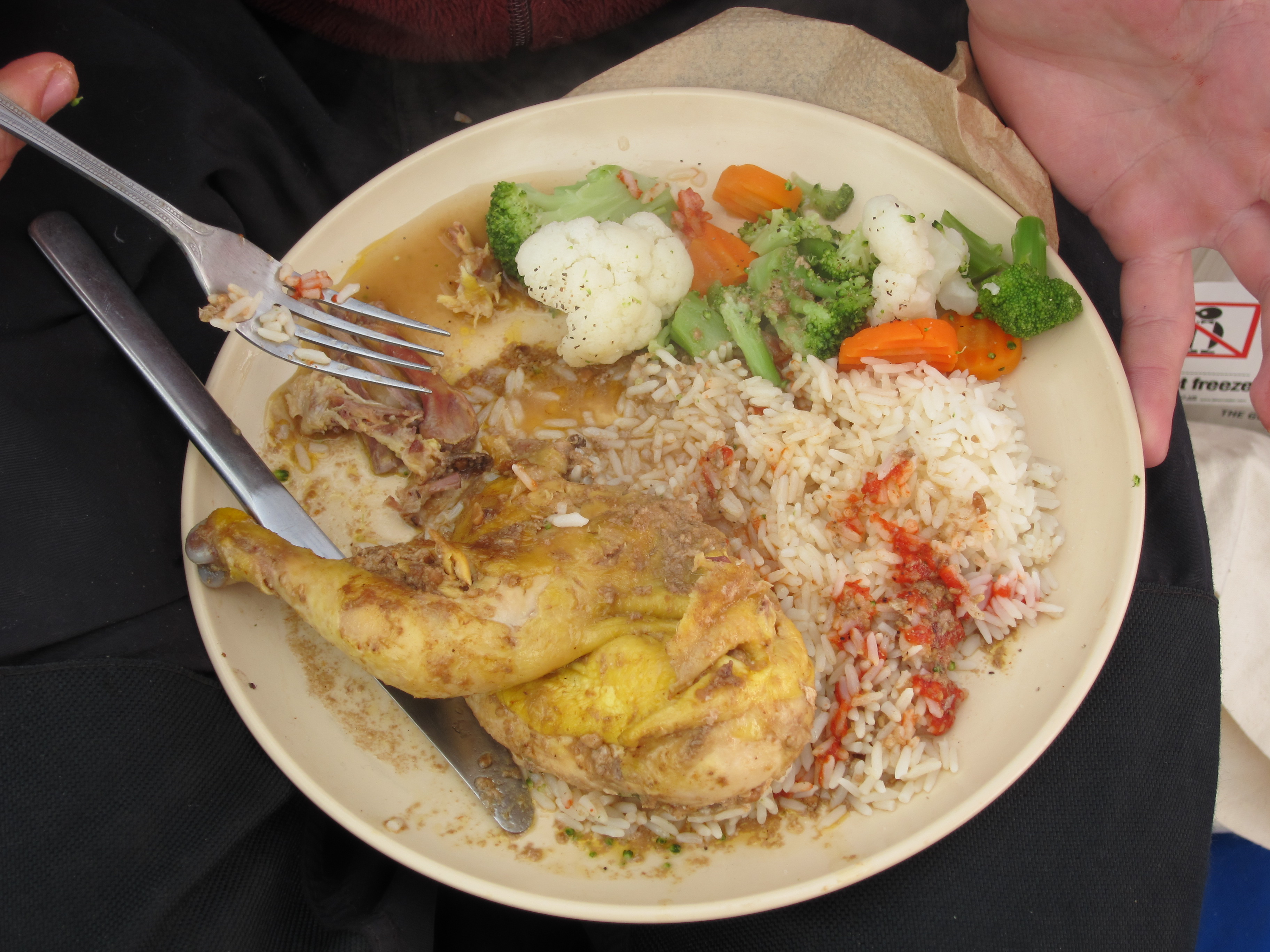
Figure 7. A delicious meal of cornish hen and steamed vegetables, all previously frozen, of course.
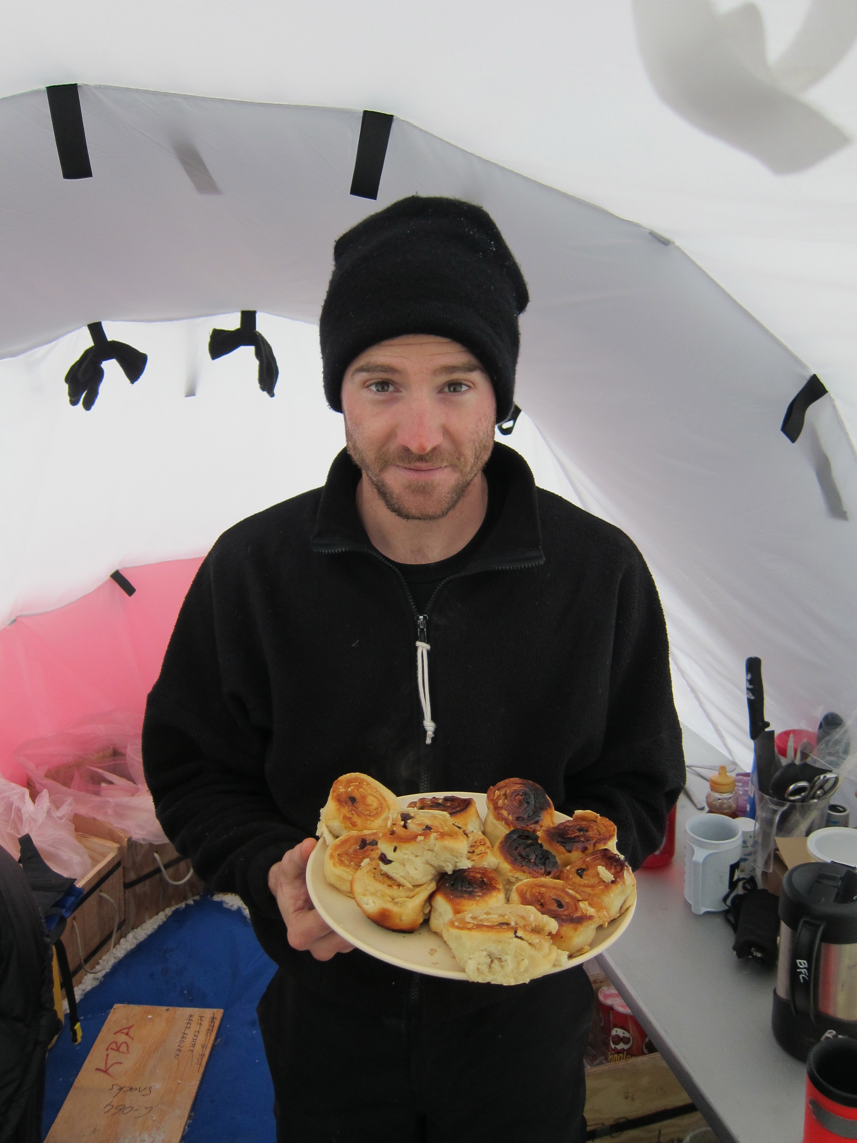
Figure 8. Cinnamon roles baked in a dutch oven on a coleman stove!
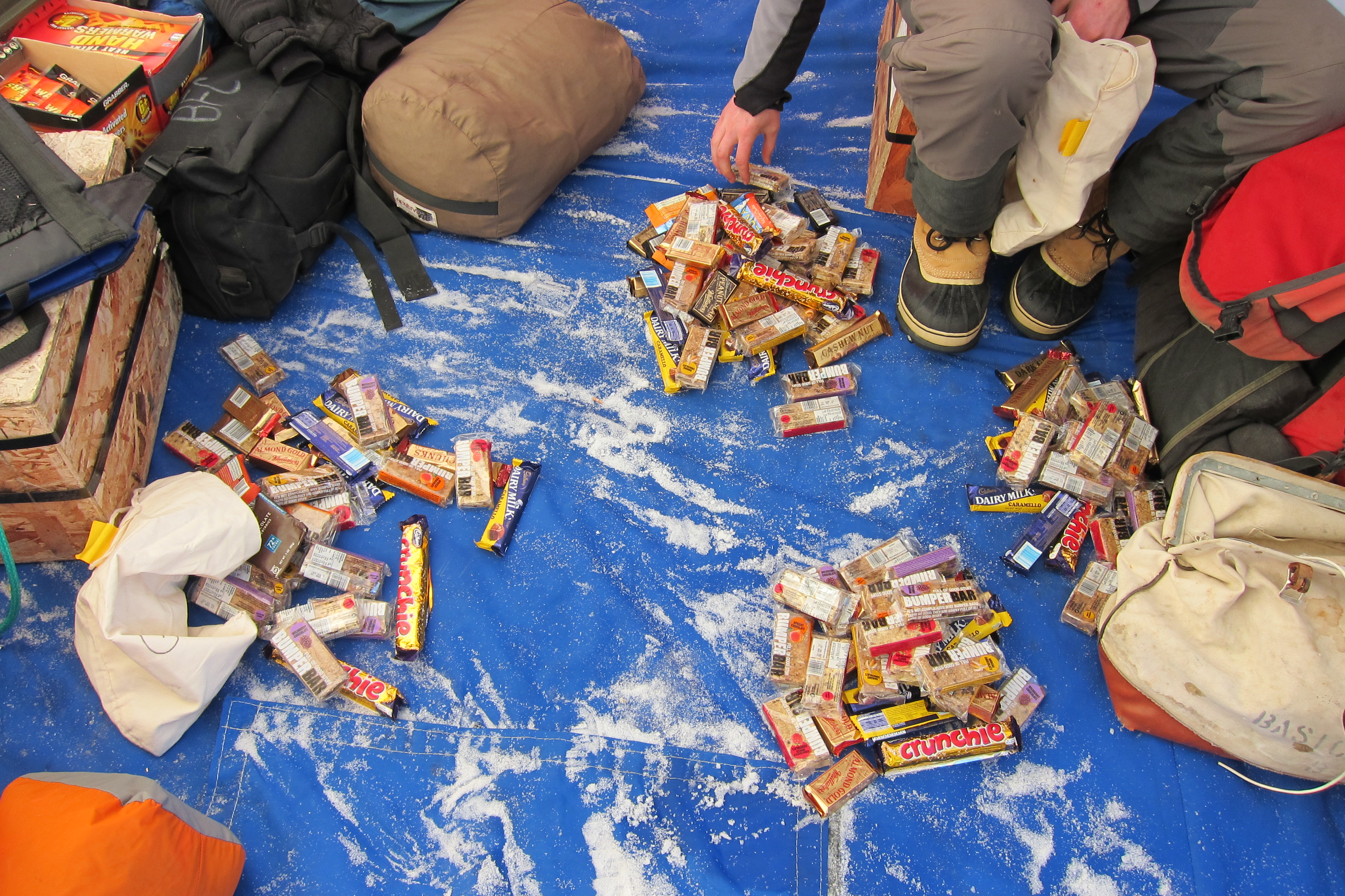
Figure 9. Dividing up the wealth of candy. Calorie-dense foods are essential as our metabolic rates increased to keep us warm!
The rocks in the field
As you can tell from the satellite image in Figure 1, snow and ice covers much of the bedrock in the Transantarctic Mountains. However, there is no vegetation and no soil, so the outcrops are excellent where they are exposed. We covered large areas with broad-scale mapping and collected hundreds of structural data and rock samples. In southern Victoria Land, beautiful multiply-deformed metasedimentary rocks host large bodies of orthogneiss and undeformed granitoids (Figs. 10–14). We focused on all of these units with detailed observations and sampling, as we are interested in the deformational, metamorphic, and igneous history of the orogen in this area. The research questions that we are exploring include: 1) What do the metamorphic rocks tell us about the timing and style of pre-magmatic tectonism? 2) Were there variations in the timing and source of magmatism along a ~450 km strike-length of the orogen? 3) Can we discern between crustal and mantle magma sources using geochemistry and radiogenic isotopes?
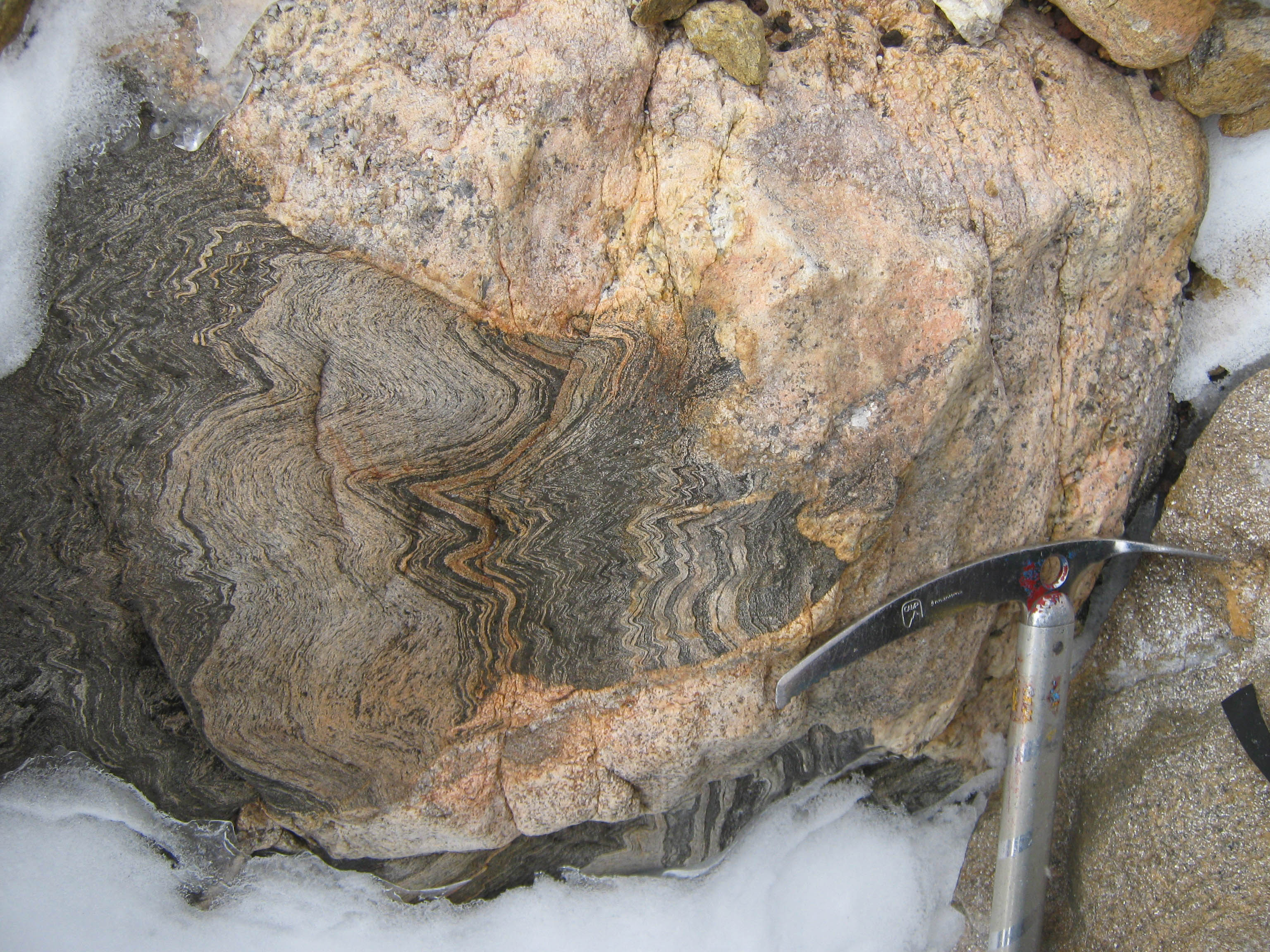
Figure 10. Folded paragneiss intruded by granite.
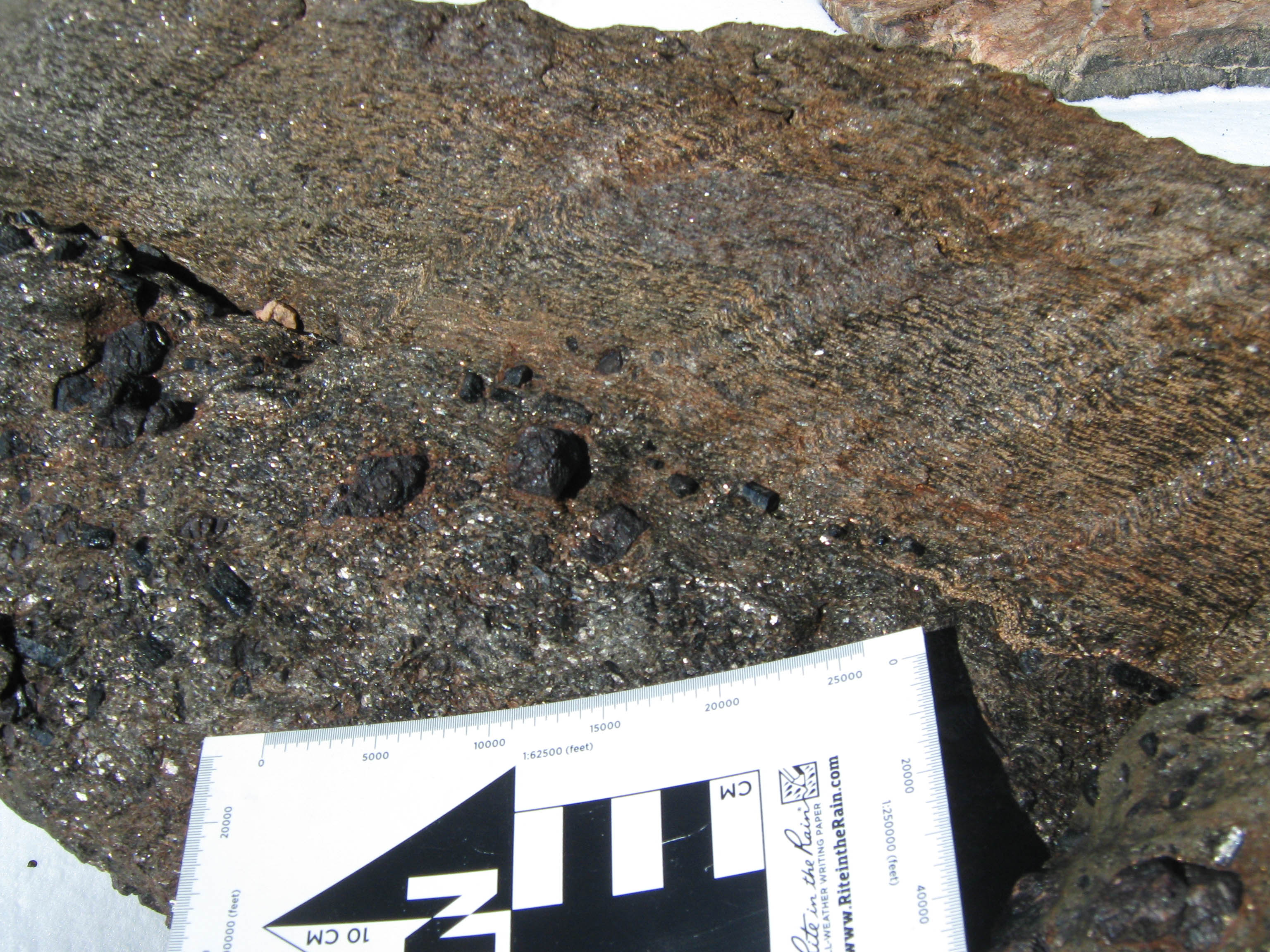
Figure 11. A sharp contact between an amphibolite and a garnet-tourmaline schist with large (>1 cm diameter) garnet porphyroblasts.
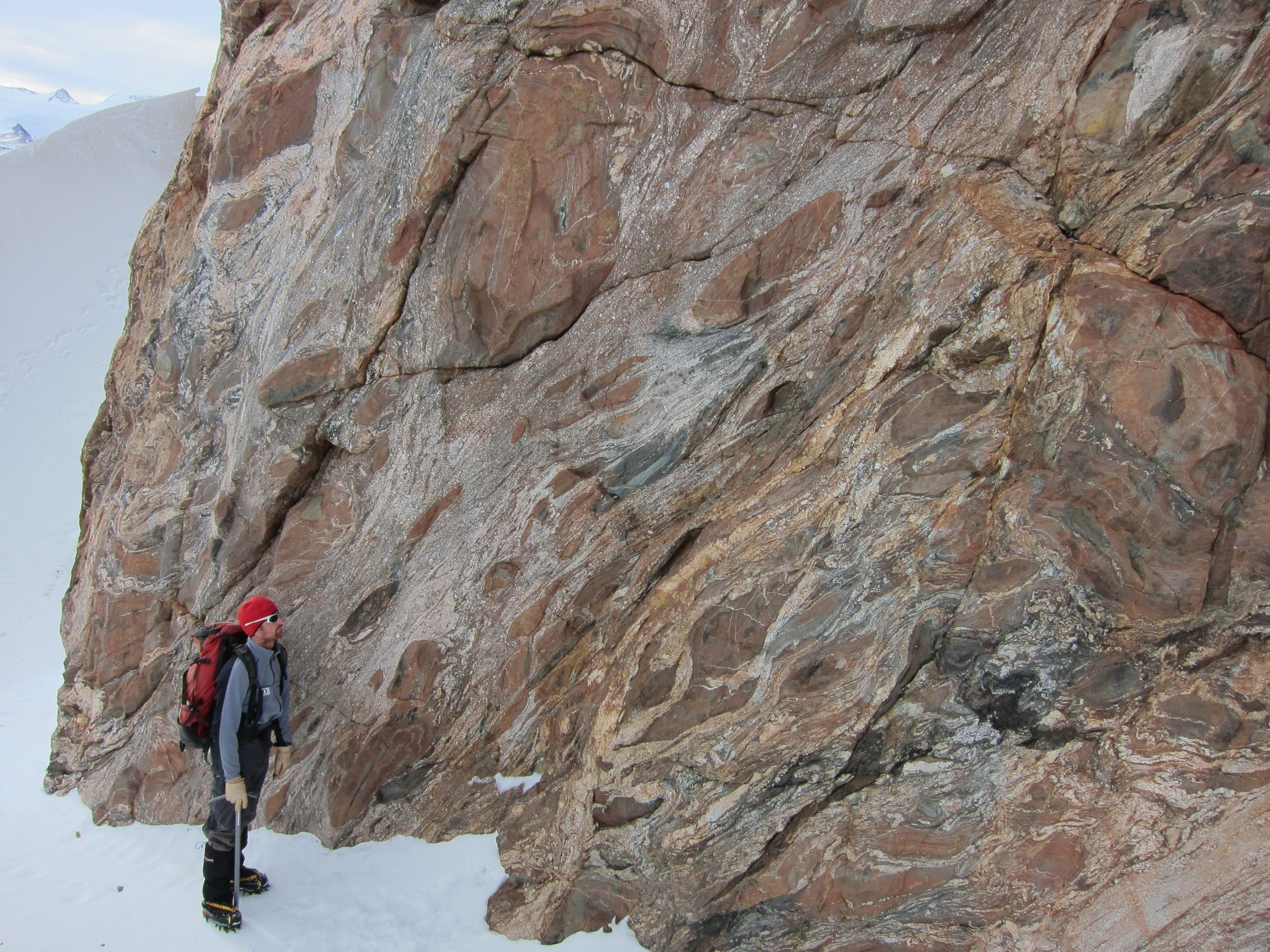
Figure 12. My supervisor, John Cottle, examines a shear zone with ellipsoidal and sigmoidal pods of paragneiss in a migmatitic matrix.
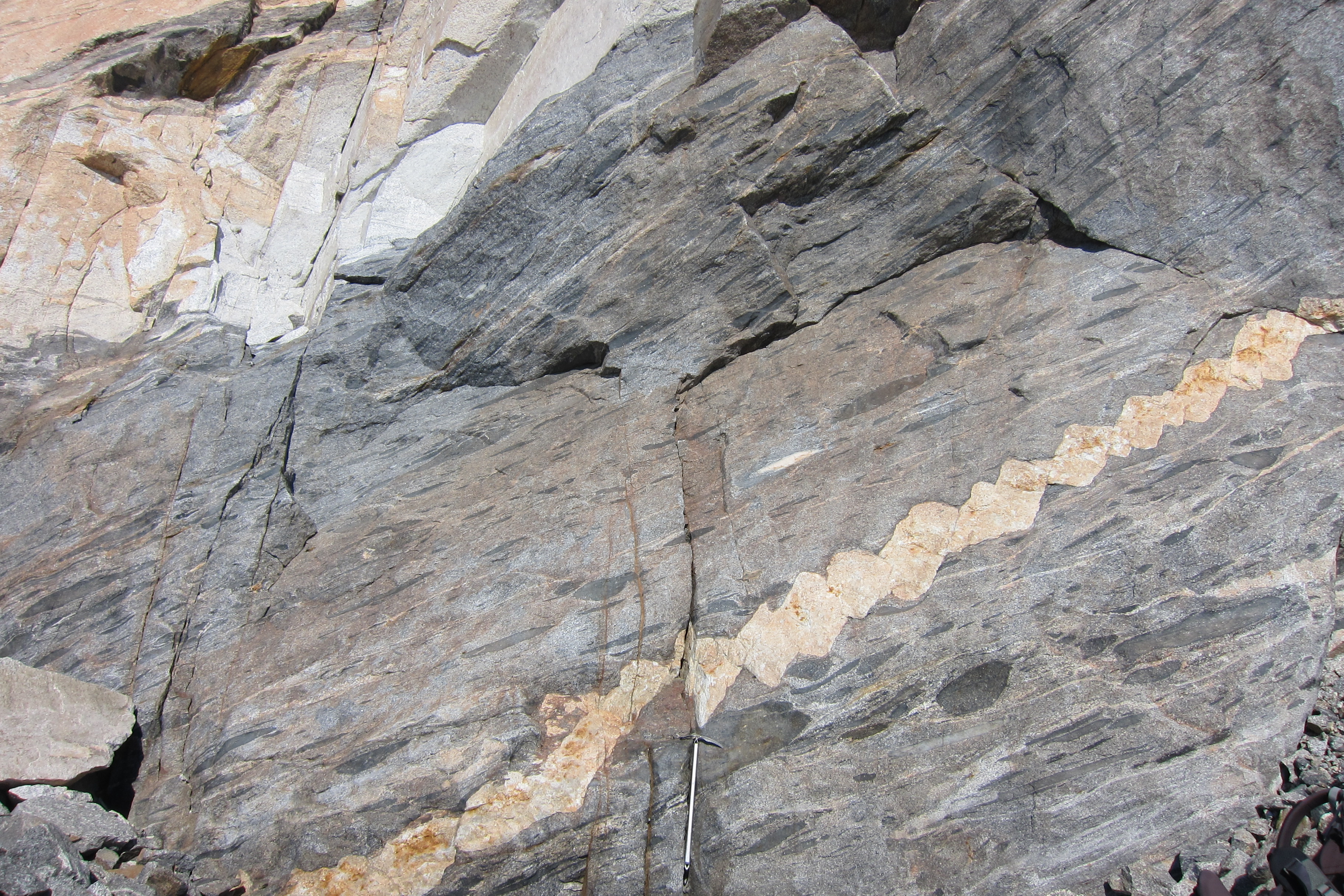
Figure 13. A dark grey orthogneiss containing strained mafic enclaves is cross-cut by a leucogranite dike that shows domino boudinage. Ice axe for scale.
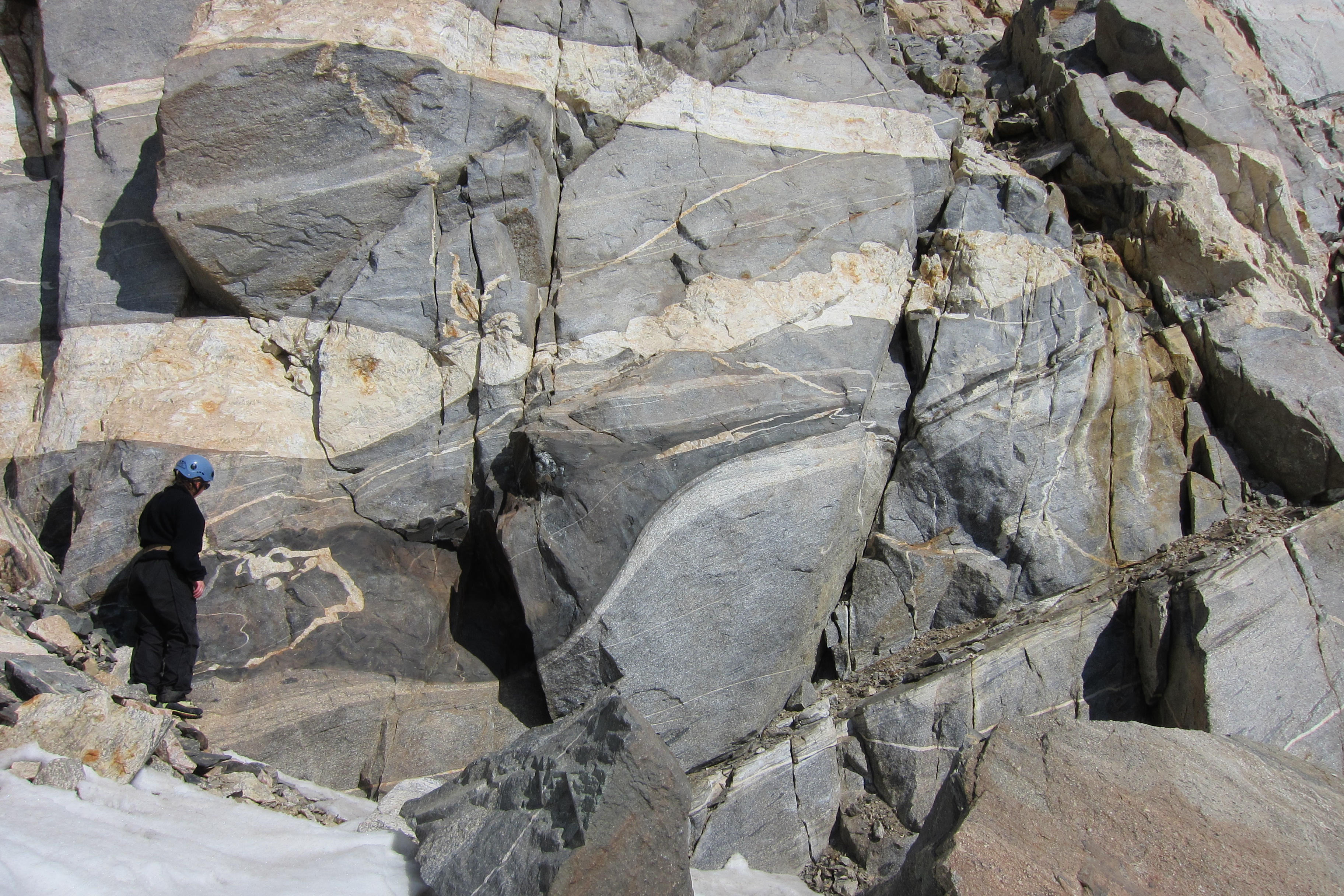
Figure 14. My friend and lab mate, Sophie Briggs, examines a pod of diorite that is enveloped in strained grey orthogneiss.
In the lab
For every amazing field season spent in a spectacular natural setting, there are countless hours spent in windowless, humming laboratories. Fortunately, I enjoy analytical work too (most of the time)! Some of the instruments that we use at UCSB include an SEM, EPMA, and laser-ablation ICP-MS (Figs. 15–17). These various tools enable us to image rocks and minerals (e.g., CL, X-ray maps, etc.) and determine the chemical and isotopic compositions of small domains in minerals (e.g., EPMA, LASS-ICP-MS). A few examples of the different types of data that we use are shown in figures 18–20. We combine petrography and whole-rock geochemistry with zircon age, isotopic, and trace element data to explore the timing and source of magmatism in the orogen. We combine thermobarometry with garnet Lu-Hf and monazite U-Th-Pb geochronology to determine the conditions and timing of metamorphism of the country rock. This multifaceted approach has revealed many details of the ca. 80 million year tectonic history of southern Victoria Land during the Ross ororgeny.
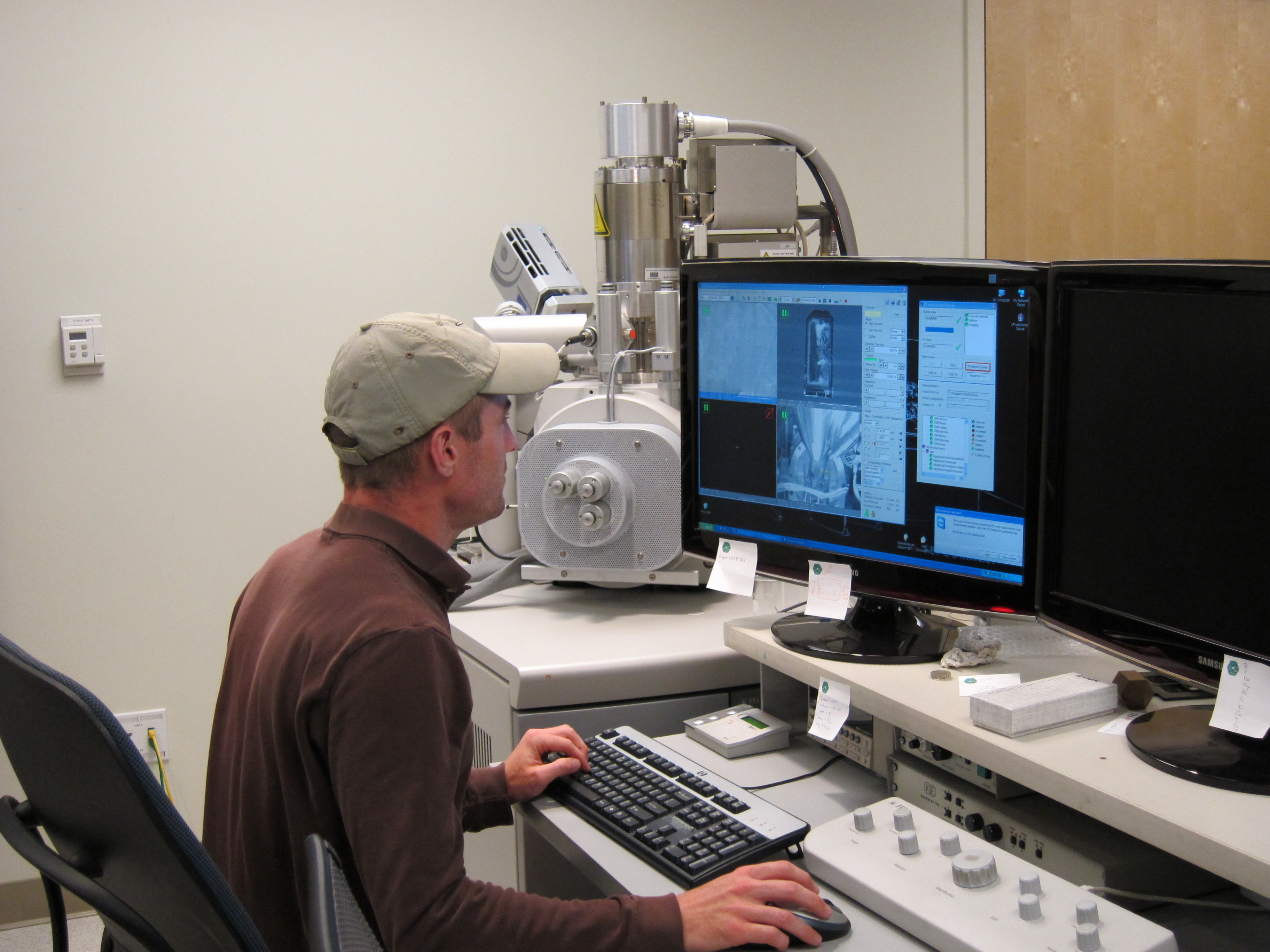
Figure 15. Generating zircon cathodoluminescence (CL) images with the SEM.
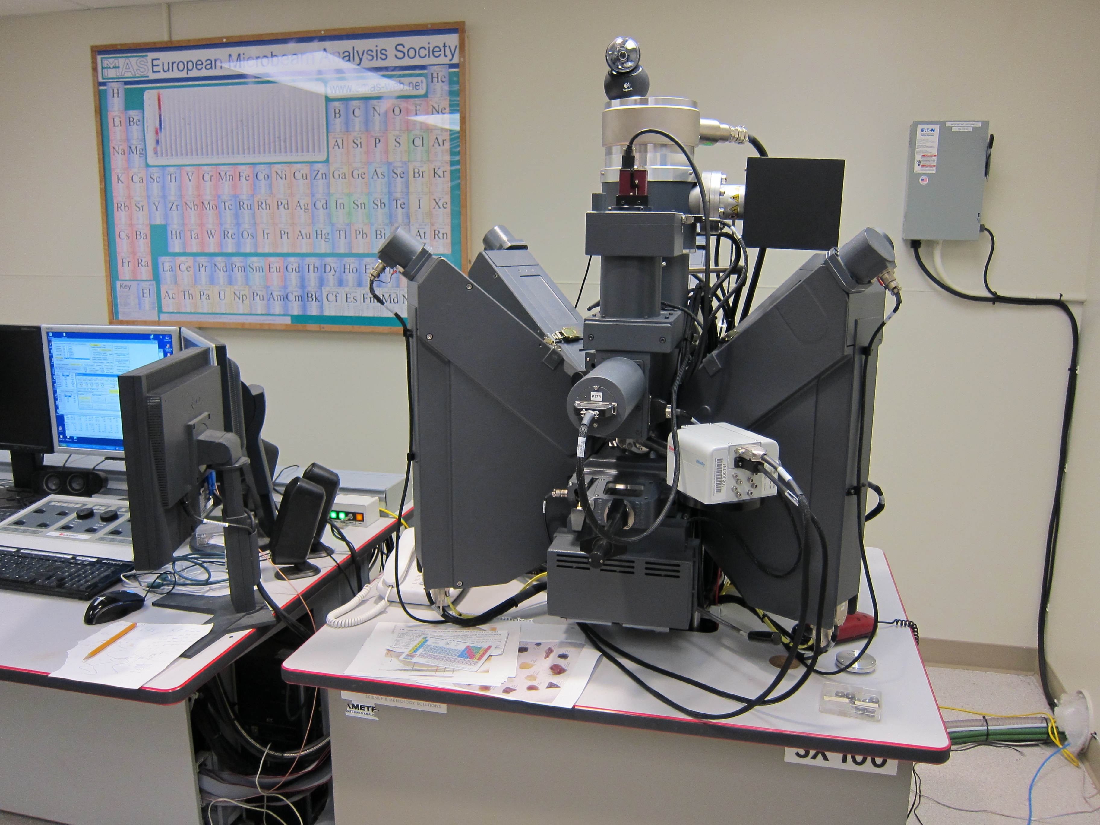
Figure 16. The electron microprobe is used for making X-ray maps and quantitative chemical analyses.

Figure 17. The ICP laboratory contains three ICP mass spectrometers (two pictured here) in one (small) room. We can connect the excimer laser to two mass spectrometers to simultaneously measure U-Th-Pb (±Hf) isotopes and trace elements in small (~10–50 μm diameter) mineral domains.
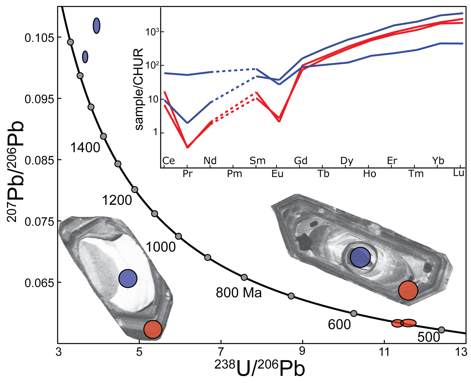
Figure 18. An example of zircon U-Pb and REE data for samples from the Byrd Glacier area. The two grains pictured have Cambrian rims with consistent REE patterns and inherited Proterozoic cores (apparent in the CL images) with distinct REE patterns. The color circles on the grains mark the locations of laser ablation pits (~25 μm diameter) and correspond to the color of the error ellipses on the Terra-Wasserburg concordia diagram.
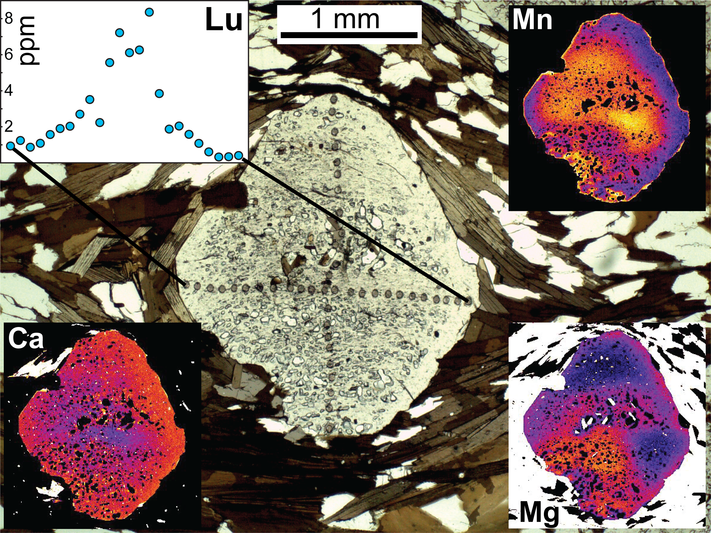
Figure 19. A photomicrograph of a garnet porphyroblast and corresponding Ca, Fe, and Mn X-ray maps. The trails of spots across the garnet are laser-ablation pits for trace element measurements. The profile of Lu concentration across one traverse is shown.
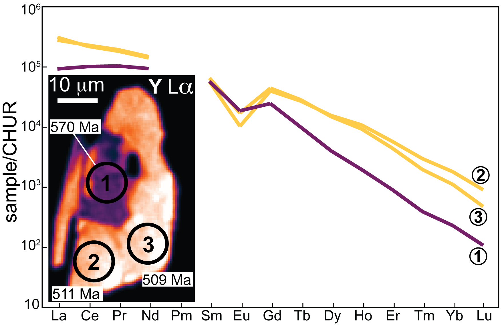
Figure 20. Combining monazite textures with age and trace element data can provide a wealth of information. The inset X-ray map shows a monazite grain with at least two distinct age/compositional domains and the locations of laser-ablation split-stream pits. The corresponding REE patterns for these analyses are also shown. The core is depleted in Y and the heavy REE relative to the rim.
Please keep an eye out for talks and papers or contact me if you would like to learn more about our research or our facilities. This work was funded by National Science Foundation grant ANT-1043152 to John M. Cottle. Please check out our websites and blog:
www.sites.google.com/site/icpgeolucsb
![]() This work is licensed under a Creative Commons Attribution-NonCommercial-ShareAlike 4.0 International License.
This work is licensed under a Creative Commons Attribution-NonCommercial-ShareAlike 4.0 International License.